深入浅出PyTorch

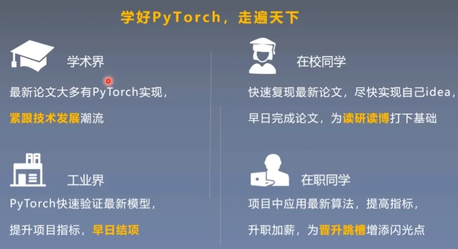
为什么要学习PyTorch？

Pytorch日益增长的发展速度与深度学习时代的迫切需要。（其实是导师项目要用这个不得不学）

---

Pytorch优点：

• 上手快：掌握Numpy和基本深度学习概念即可上手

• 代码简洁灵活：用nn.module封装使网络搭建更方便；基于动态图机制，更灵活

• Debug方便：调试PyTorch就像调试Python代码一样简单
• 文档规范：https://pytorch.org/docs/可查各版本文档

• 资源多：arXiv中的新算法大多有PyTorch实现

• 开发者多：GitHub上贡献者（Contributors）已超过1350+

• 背靠大树：FaceBook维护开发

---

学习Pytorch收益：

---

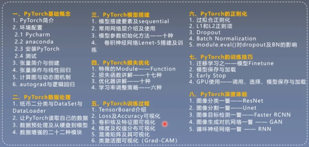
Pytorch学习哪些知识

Pytorch定位：深度学习框架，实现深度学习模型算法

人工智能：多领域交叉科学技术

机器学习：计算机智能决策算法

深度学习：高效的机器学习算法

---

Pytorch实现模型训练

模型训练过程中细分的过程：

---

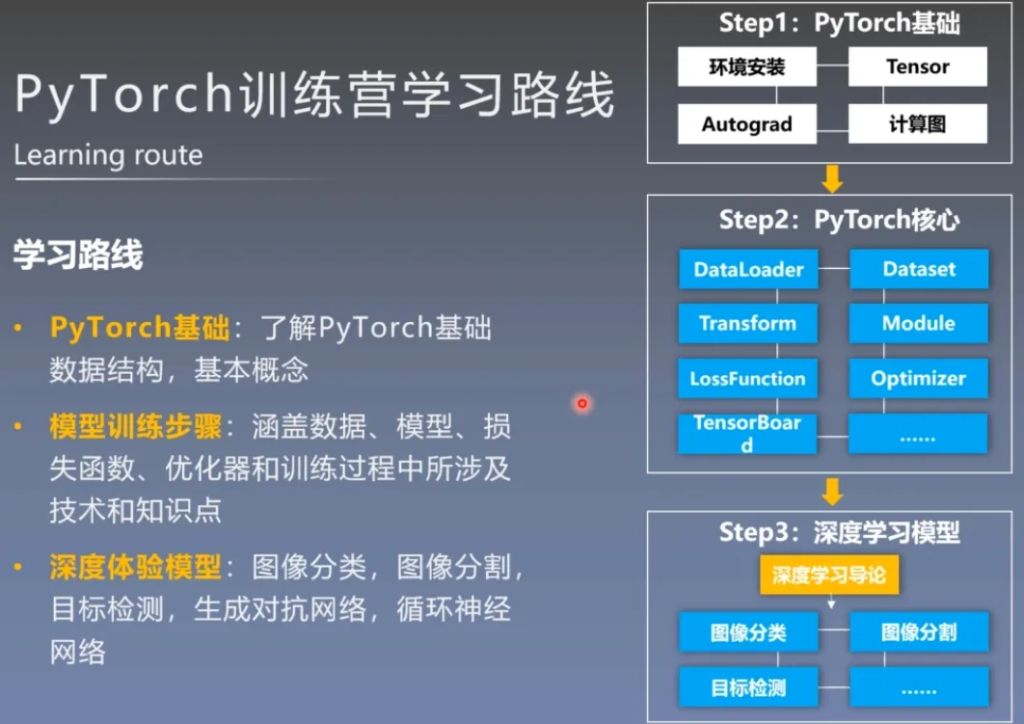
如何学习和掌握Pytorch

学习Pytorch的困境

跟课、多思考、多实践、多问大模型、多总结

---

Pytorch学习路径

整个课程大致的学习内容

---

Pytorch学习路线

---

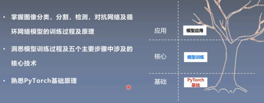
最终能达到的目标

---

Pytorch简介与安装

Pytorch简介

简而言之，Pytorch是在Torch基础上用python语言重新打造的深度学习框架。

Pytorch发展迅速，在深度学习领域占比增长速度很快。

这些在上面已经说明了很多，这里不多赘述了。

---

软件安装（环境配置与搭建）

解释器与工具包

解释器：将python语言翻译成机器指令语言的程序

工具包：又称之为依赖包、模块、库、包等

• python之所以强大是因为拥有大量工具包
• 内置包：os、sys、glob、re、math等
• 第三方包：pytorch、TensorFlow、numpy等

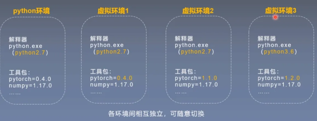
虚拟环境

在python开发环境中，有python解释器与工具包。

在不同项目中，采用的解释器版本与工具包版本可能不同。

所以我们为项目创建虚拟环境来满足需求，各环境间相互独立，可以随意切换

Anaconda

Anaconda是为方便使用python而建立的一个软件包，其包含了常用的250多个工具包，多版本python解释器和强大的虚拟环境管理工具。

Anaconda可以使安装、运行和升级环境变得简单，因此推荐使用。

安装步骤：

1. Https://www.anaconda.com/distribution/#download-section官网下载安装包
2. 运行Anaconda3-2019.07-Windows-x86 64.exe
3. 选择路径，勾选将Add Anaconda to the system PATH environment variable，等待安装完成
4. 验证安装成功，打开命令、输入Conda、回车
5. 添加中科大镜像

Pycharm（可以使用VScode）

Pycharm是一款python的IDE，总之功能强大就对了。

安装步骤：

1. 官网下载安装包https://www.jetbrains.com/pycharm/

2. 运行pycharm-professional-2019.2.exe

3. 选择路径，勾选Add launchers dir to the PATH，等待安装完成

Pytorch

安装步骤：

1. 检查是否有合适GPU，若有，需安装CUDA与CuDNN
2. CUDA与CuDNN安装（非必须）
3. 下载whl文件，登陆https://download.pytorch.org/whl/torch_stable.html，下载pytorch与torchvision的whl文件，进入相应虚拟环境，通过pip安装
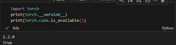
4. 在pycharm中创建hellopytorch项目，运行脚本，查看pytorch版本

命名解释：

cu92/torch-1.2.0%2Bcu92-cp37-cp37m-win_amd64.whl

Anaconda创建虚拟环境

需要新建一个环境可以起名叫做DL（其他也行）

conda create -n DL python=3.8
conda env list
conda activate DL
conda install jupyter
pip insatll scikit-learn

---

以上全部可以看CSDN上详细的步骤：

【超详细教程】2024最新Pytorch安装教程（同时讲解安装CPU和GPU版本）-CSDN博客

程序输出一下

---

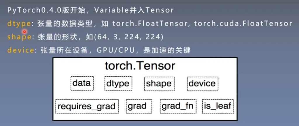
Pytorch的Tensor（张量）

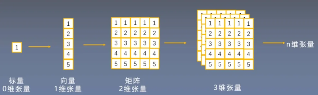
张量是什么？

张量在数学概念中是一个多维数组，它是标量、向量、矩阵的高维拓展

Tensor与Variable

variable主要是给Tensor增加了四个属性，这四个属性用于自动求导

---

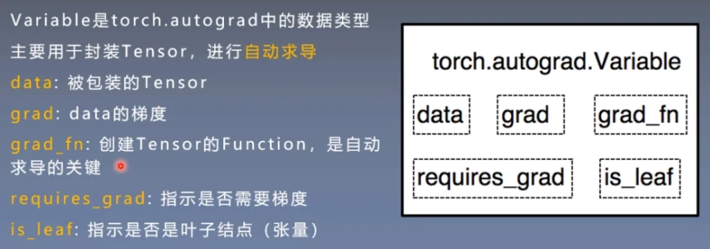
Tensor

下方的四个在Variable中介绍过了，与求导相关的。

---

张量的创建

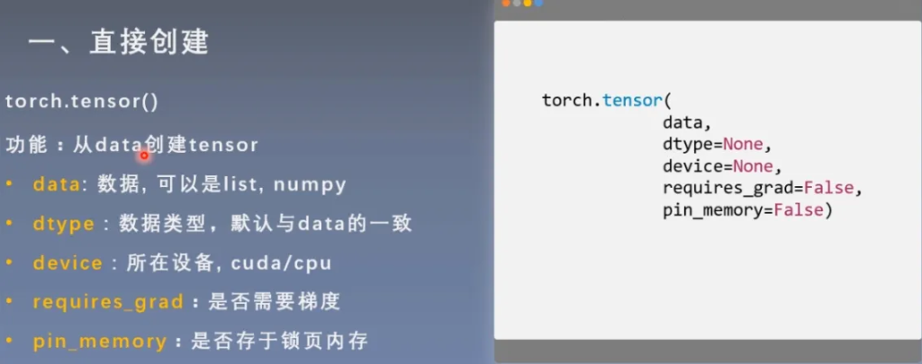
1 直接创建

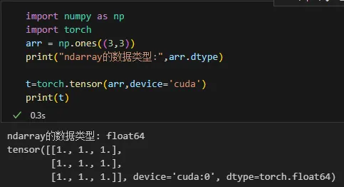
从data创建tensor

import numpy as np
import torch
arr = np.ones((3,3))
print("ndarray的数据类型:",arr.dtype)

t=torch.tensor(arr,device='cuda')
print(t)

结果：

---

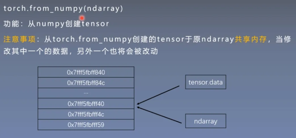
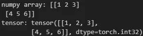
从numpy创建tensor

注意：通过这样方式创建的tensor与原ndarray共享内存

import numpy as np
import torch
arr = np.array([[1,2,3],[4,5,6]])

t=torch.from_numpy(arr)
print("numpy array:",arr)
print("tensor:",t)

结果：

---

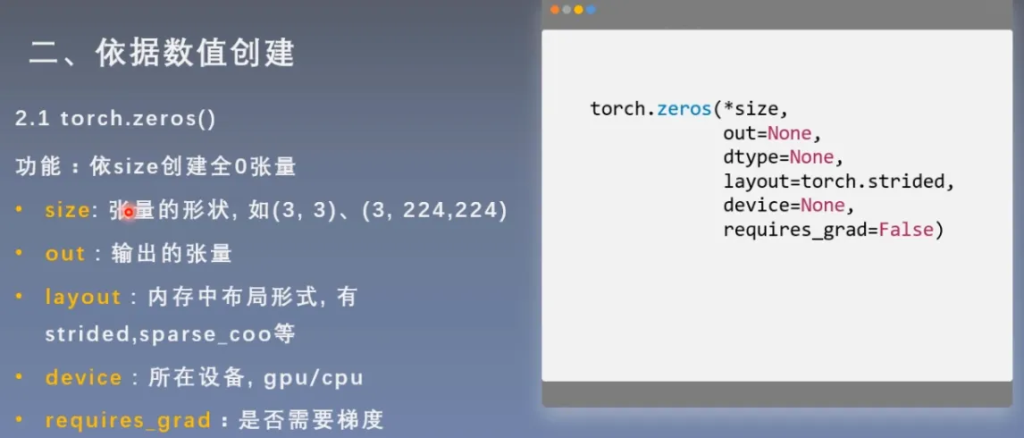
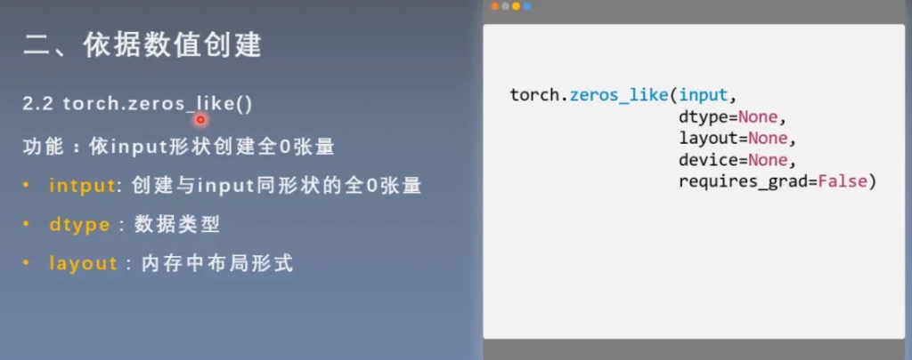
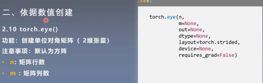
2 依据数值创建

依据数值创建全0张量

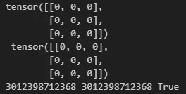
由代码我们可以得知，我们创建的t赋值给了out_t

import torch

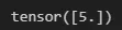
out_t = torch.tensor([1])

t = torch.zeros((3,3),out=out_t)

print(t,'\n',out_t)
print(id(t,),id(out_t),id(t)==id(out_t))

结果：

---

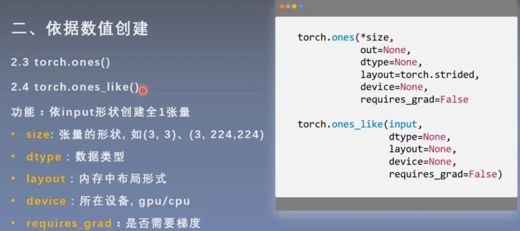
依据数值创建全1张量

这里ones与上面是类似的

pytorch还给我们提供了填充任意值的函数

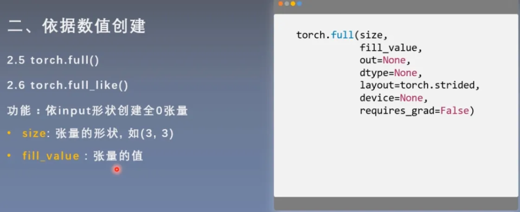
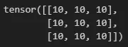
import torch

t = torch.full((3,3),10)
print(t)

结果：

---

创建等差数列的张量

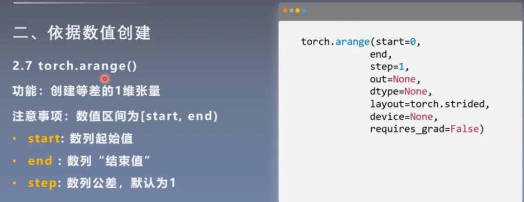
import torch

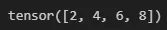
t = torch.arange(2,10,2)
print(t)

结果：

---

创建均分数列的张量

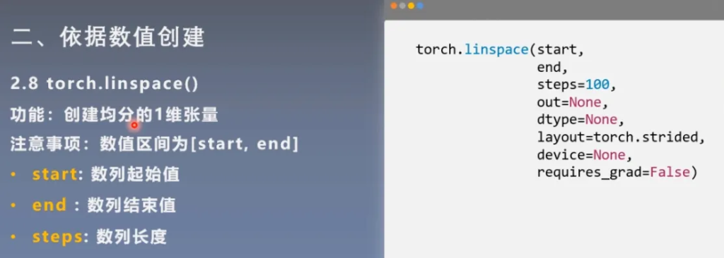
import torch

t = torch.linspace(2,10,5)
print(t)

结果：

---

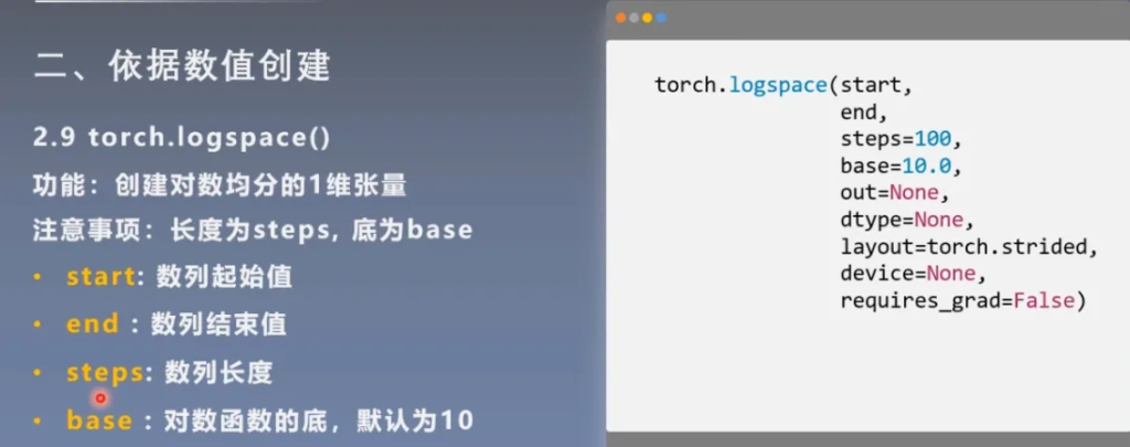
创建对数均分的张量

---

创建单位对角矩阵张量

---

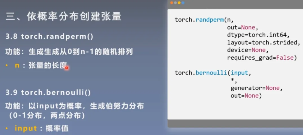
3 依据概率分布创建张量

正态分布

也称为高斯分布

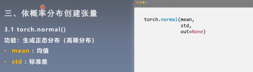
四种模式：

• mean为标量，std为标量
• mean为标量，std为张量
• mean为张量，std为标量
• mean为张量，std为张量

import torch
#mean:张量 std:张量
# mean = torch.arange(1,5,dtype=torch.float)
# std = torch.arange(1,5,dtype=torch.float)
# t_normal = torch.normal(mean,std)
# print("mean:{}\nstd:{}".format(mean,std))
# print(t_normal)

#mean:标量 std:标量
# t_normal = torch.normal(0., 1., size=(4,))
# print(t_normal)

#mean:张量 std:标量
# mean = torch.arange(1,5,dtype=torch.float)
# std = 1
# t_normal = torch.normal(mean,std)
# print("mean:{}\nstd:{}".format(mean,std))
# print(t_normal)

---

标准正态分布

---

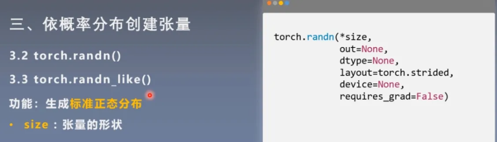
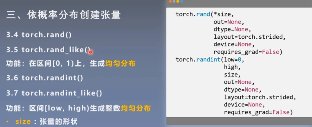
均匀分布

---

随机排列和概率值

---

张量的操作与线性回归

张量的操作

拼接

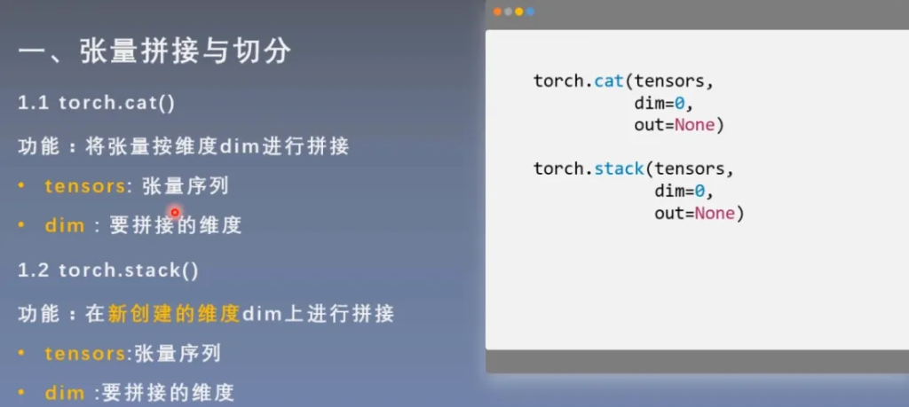
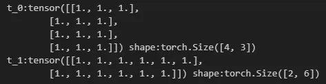
import torch

t = torch.ones((2,3))

t_0 = torch.cat([t,t],dim=0)
t_1 = torch.cat([t,t],dim=1)

print("t_0:{} shape:{}".format(t_0,t_0.shape))
print("t_1:{} shape:{}".format(t_1,t_1.shape))

结果：

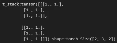
import torch
t=torch.ones((2,3))
t_stack=torch.stack([t,t],dim=2)
print("t_stack:{} shape:{}".format(t_stack,t_stack.shape))

结果：

---

切分

平均切分

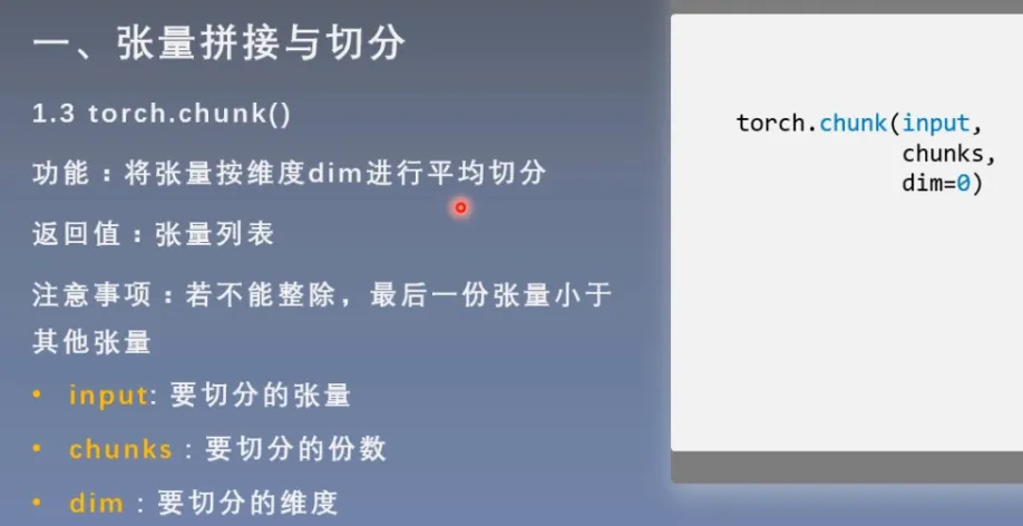
import torch

a = torch.ones((2,5))
list_of_tensors = torch.chunk(a,dim=1,chunks=2)

for idx,t in enumerate(list_of_tensors):
    print("第{}个张量：{} shape is{}".format(idx+1,t,t.shape))

结果：

---

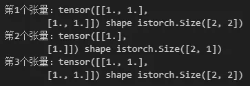
可以指定切分长度

import torch
t=torch.ones((2,5))
t=torch.ones((2,5))

list_of_tensors = torch.split(t,[2,1,2],dim=1)

for idx,t in enumerate(list_of_tensors):
    print("第{}个张量：{} shape is{}".format(idx+1,t,t.shape))

结果：

---

索引

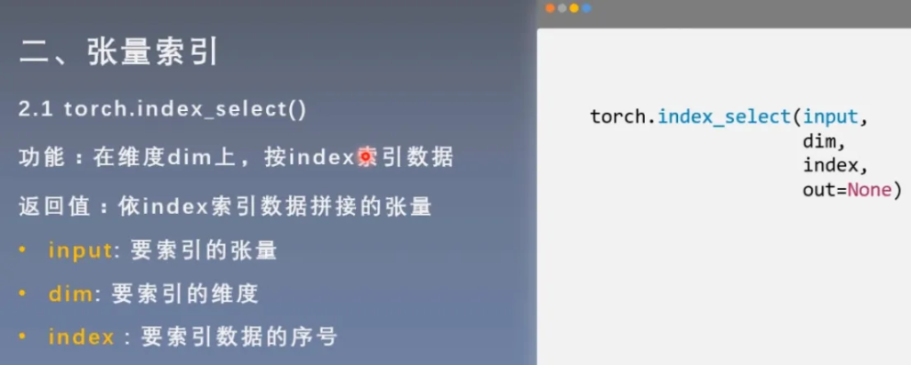
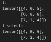
import torch

t = torch.randint(0,9,size=(3,3))
idx = torch.tensor([0,2],dtype=torch.long)
t_select = torch.index_select(t,dim=0,index=idx)
print("t:\n{}\nt_select:\n{}".format(t,t_select))

结果：

---

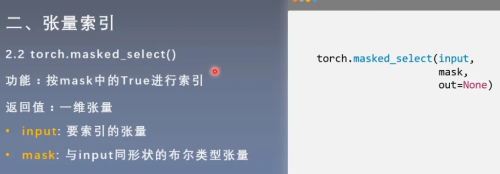
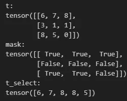
import torch

t = torch.randint(0,9,size=(3,3))
mask = t.ge(5) #大于等于5的元素为True
t_select = torch.masked_select(t,mask)

print("t:\n{}\nmask:\n{}\nt_select:\n{}".format(t,mask,t_select))

结果：

---

变换

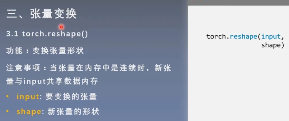
import torch

t=torch.randperm(8)
t_reshape = torch.reshape(t,(2,4))
print("t:{}\nt_reshape:\n{}".format(t,t_reshape))

t[0]=1024
print("\nt:{}\nt_reshape:\n{}".format(t,t_reshape))
print("t.data 内存地址：{}",format(id(t.data)))
print("t_reshape.data 内存地址：{}",format(id(t_reshape.data)))

结果：

---

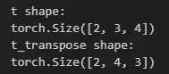
import torch
t = torch.rand((2,3,4))
t_transpose = torch.transpose(t,1,2)

print("t shape:\n{}\nt_transpose shape:\n{}".format(t.shape,t_transpose.shape))

结果：

---

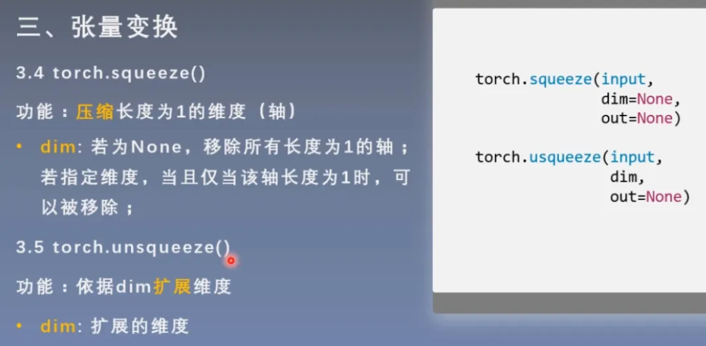
import torch
t = torch.rand((1,2,3,1))

t_sq = torch.squeeze(t)
t_0 = torch.squeeze(t,0)
t_1 = torch.squeeze(t,1)

print(t.shape)
print(t_sq.shape)
print(t_0.shape)
print(t_1.shape)

结果：

---

张量的数学运算

简单介绍一下有哪些运算，用到的时候随时查就可以了。

加减乘除

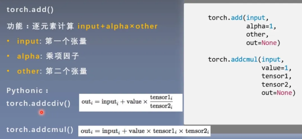
torch.add()
torch.addcdiv()
torch.addcmul()
torch.sub()
torch.div()
torch.mul()

由于我们经常用到 乘项因子x张量+张量，所以为了简洁代码，在add中内置了这样的计算。

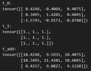
import torch

t_0 = torch.randn((3,3))
t_1 = torch.ones_like(t_0)
t_add = torch.add(t_0, 10, t_1)

print("t_0:\n{}\nt_1:\n{}\nt_add:\n{}".format(t_0,t_1,t_add))

结果：

对数，指数，幂函数

torch.log(input, out=None)
torch.log10(input, out=None)
torch.log2(input, out=None)
torch.exp(input, out=None)
torch.pow()

三角函数

torch.abs(input, out=None)
torch.acos(input, out=None)
torch.cosh(input, out=None)
torch.cos(input, out=None)
torch.asin(input, out=None)
torch.atan(input, out=None)
torch.atan2(input, other, out=None)

---

线性回归

线性回归是分析一个变量与另一（多）个变量之间关系的方法

因变量：y 自变量：x 关系：线性

y = wx + b

分析：求解w，b

---

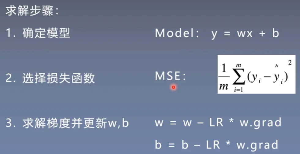
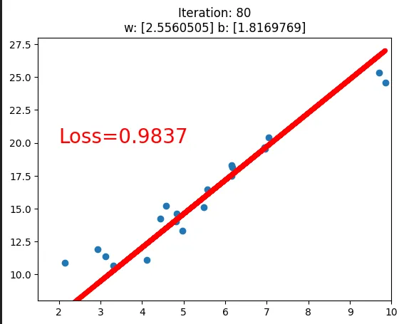
以下是代码实现：

import torch
import matplotlib.pyplot as plt
torch.manual_seed(10)

lr = 0.05  # 学习率    20191015修改

# 创建训练数据
x = torch.rand(20, 1) * 10  # x data (tensor), shape=(20, 1)
y = 2*x + (5 + torch.randn(20, 1))  # y data (tensor), shape=(20, 1)

# 构建线性回归参数
w = torch.randn((1), requires_grad=True)
b = torch.zeros((1), requires_grad=True)

for iteration in range(1000):

    # 前向传播
    wx = torch.mul(w, x)
    y_pred = torch.add(wx, b)

    # 计算 MSE loss
    loss = (0.5 * (y - y_pred) ** 2).mean()

    # 反向传播
    loss.backward()

    # 更新参数
    b.data.sub_(lr * b.grad)
    w.data.sub_(lr * w.grad)

    # 清零张量的梯度  
    w.grad.zero_()
    b.grad.zero_()

    # 绘图
    if iteration % 20 == 0:

        plt.scatter(x.data.numpy(), y.data.numpy())
        plt.plot(x.data.numpy(), y_pred.data.numpy(), 'r-', lw=5)
        plt.text(2, 20, 'Loss=%.4f' % loss.data.numpy(), fontdict={'size': 20, 'color':  'red'})
        plt.xlim(1.5, 10)
        plt.ylim(8, 28)
        plt.title("Iteration: {}\nw: {} b: {}".format(iteration, w.data.numpy(), b.data.numpy()))
        plt.pause(0.5)

        if loss.data.numpy() < 1:
            break

结果：在迭代80次后loss降到了1以下

---

这部分还不是很懂，回头补充一下。

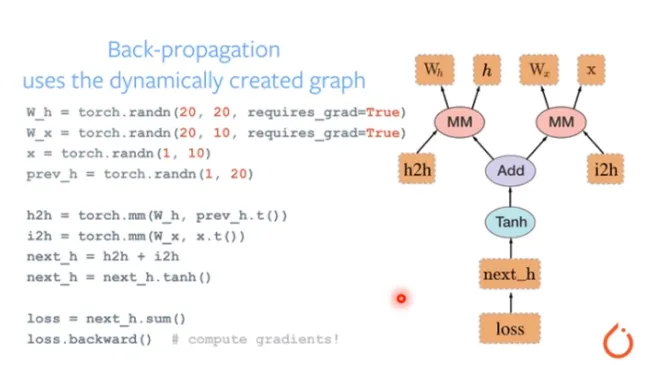
计算图与动态图机制

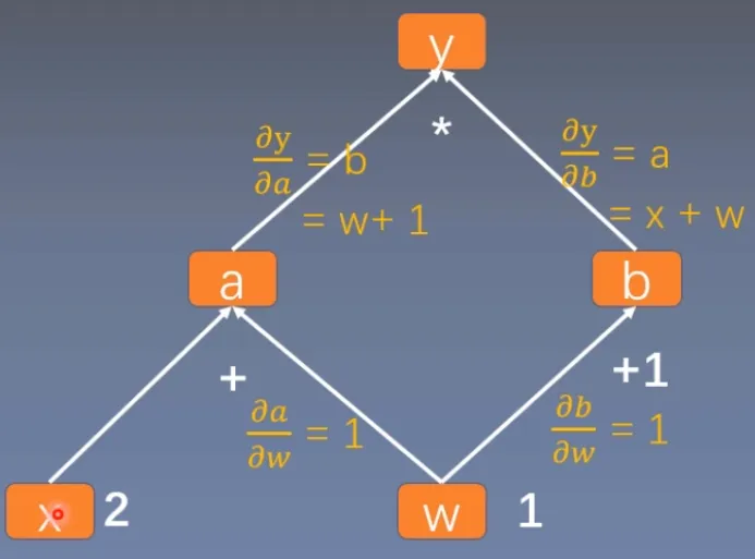
计算图

计算图是用来描述运算的有向无环图

计算图有两个主要元素：结点（Node） 边（Edge）

结点表示数据，如向量、矩阵、张量

边表示运算，如加减乘除卷积等

用计算图表示：y = (x + w) * (w + 1)

---

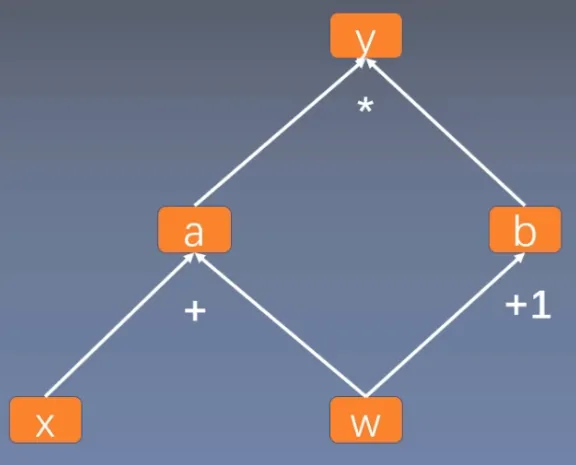
使用计算图不仅仅可以让计算变得简洁，更重要的作用是使得梯度求导变得更加方便

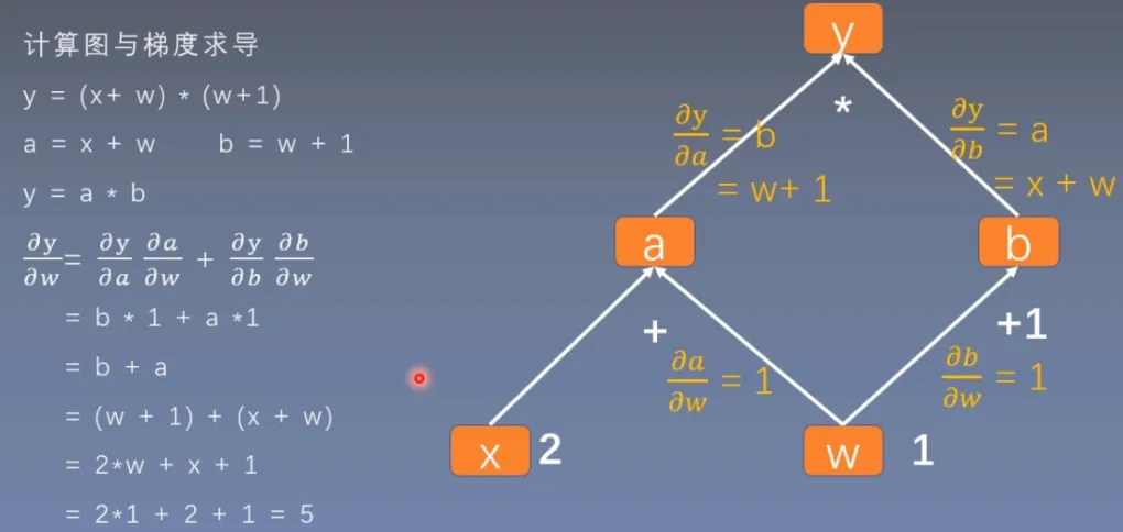
用代码来验证一下：

import torch

w = torch.tensor([1.], requires_grad=True)
x = torch.tensor([2.], requires_grad=True)

a = torch.add(w, x)     # retain_grad()
b = torch.add(w, 1)
y = torch.mul(a, b)

y.backward()
print(w.grad)

结果：

---

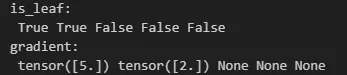
is_leaf

在之前学习张量时，Tensor中有is_leaf的变量，用来指示张量是否为叶子结点。

同时非叶子结点在反向传播后，其梯度会被释放掉。

如果想要保留非叶子结点的梯度，需要加上retain_grad( )

# 查看叶子结点
print("is_leaf:\n", w.is_leaf, x.is_leaf, a.is_leaf, b.is_leaf, y.is_leaf)

# 查看梯度
print("gradient:\n", w.grad, x.grad, a.grad, b.grad, y.grad)

结果：

---

grad_fn

用来记录创建该张量时所用的方法（函数），用来在反向传播时计算梯度。

y.grad_fn =<MulBackward0>

a.grad_fn =<AddBackward0>

b.grad_fn =<AddBackward0>

# 查看 grad_fn
print("grad_fn:\n", w.grad_fn, x.grad_fn, a.grad_fn, b.grad_fn, y.grad_fn)

结果：

---

动态图

根据计算图搭建方式，可将计算图分为动态图和静态图

动态图：运算与搭建同时进行（Pytorch）

静态图：先搭建图，后运算（TensorFlow）

Pytorch是在每一步计算的同时搭建图

而Tensorflow是先搭建好所有的图，再传入数据进行计算

---

Autograd与逻辑回顾

torch.autograd—自动求导系统

backward

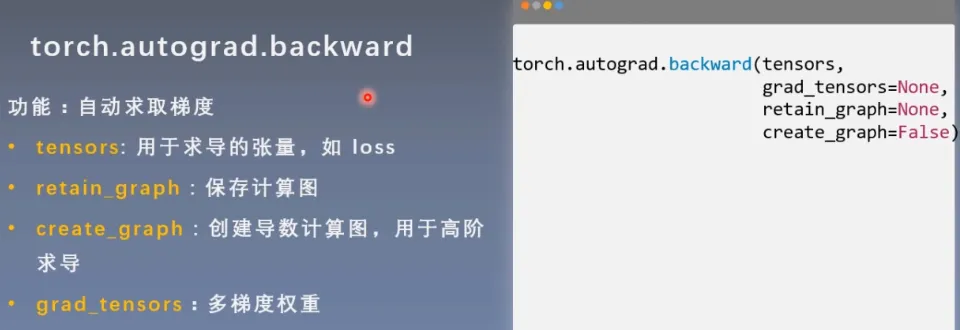
grad

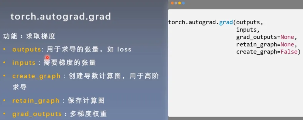
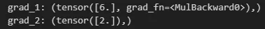
import torch

x = torch.tensor([3.],requires_grad=True)
y = torch.pow(x,2)

#创建图，为了计算二阶导数
grad_1 = torch.autograd.grad(y,x,create_graph=True)
print("grad_1:",grad_1)

grad_2 = torch.autograd.grad(grad_1[0],x)
print("grad_2:",grad_2)

结果：

---

autograd小贴士：

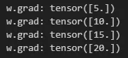
1. 梯度不自动清零

import torch

w = torch.tensor([1.], requires_grad=True)
x = torch.tensor([2.], requires_grad=True)

for i in range(4):
    a = torch.add(w, x)     # retain_grad()
    b = torch.add(w, 1)
    y = torch.mul(a, b)

    y.backward()

    print("w.grad:", w.grad)

    #w.grad.zero_()

结果：

2. 依赖于叶子结点的结点，requires_grad默认为True

可以用这张图来理解，a的梯度依赖于x的梯度，所以其requires_grad默认为True

import torch

w = torch.tensor([1.], requires_grad=True)
x = torch.tensor([2.], requires_grad=True)

a = torch.add(w, x)     # retain_grad()
b = torch.add(w, 1)
y = torch.mul(a, b)


print(a.requires_grad,b.requires_grad,y.requires_grad)

结果：

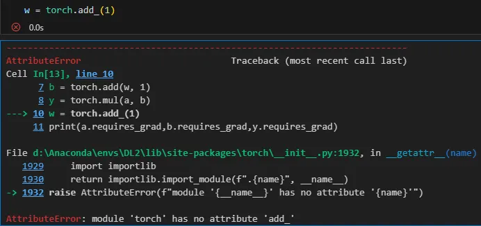
3. 叶子结点不可执行in-place（原地操作）

在前向传播过程中，会记录叶子结点的地址；在反向传播过程中，根据地址去寻找叶子结点的值，如果这个时候叶子结点原地操作导致值的改变，就与前向传播过程中的值不同，这就会产生错误。

import torch

w = torch.tensor([1.], requires_grad=True)
x = torch.tensor([2.], requires_grad=True)

a = torch.add(w, x)     # retain_grad()
b = torch.add(w, 1)
y = torch.mul(a, b)

w = torch.add_(1)

结果：

---

逻辑回归

什么是逻辑回归模型？

逻辑回归模型是线性的二分类模型

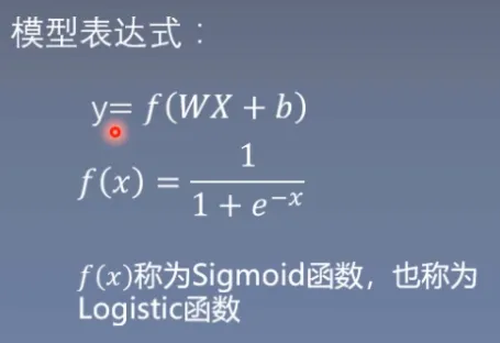
sigmoid函数：将输入的数据映射到0到1之间

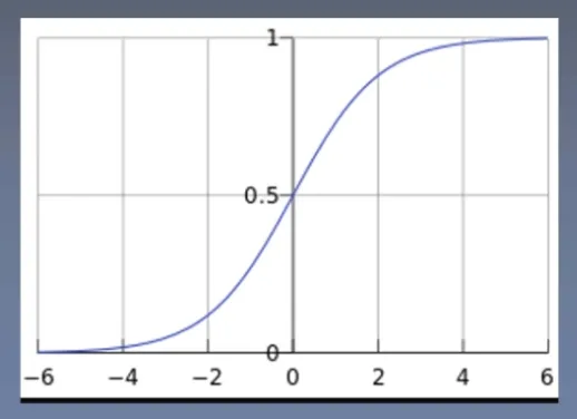
二分类：设置一个阈值为0.5，当y<0.5为0，当y>=0.5为1

线性：

逻辑回归模型相当于在线性回归模型的基础上增加了一个激活函数

即便没有这个激活函数，线性回归模型也可以做二分类问题，等价于y>0则为1，y<0为0

但是为了更好的描述分类自信度，我们将值映射到01之间，符合概率取值

---

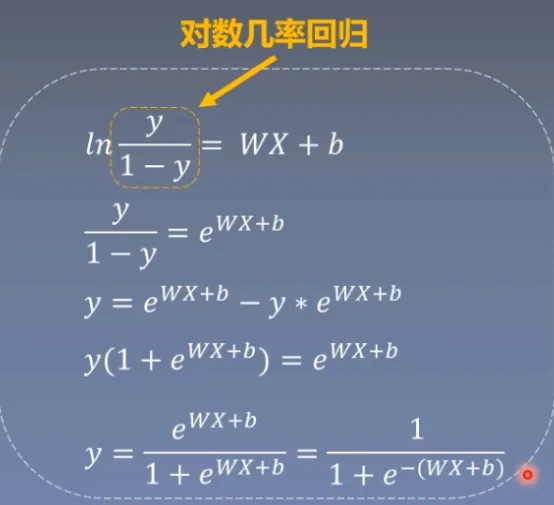
逻辑回归也可以叫 对数几率回归

---

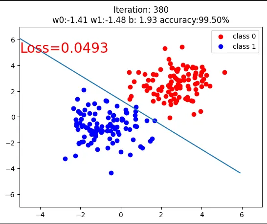
模型训练过程

import torch
import torch.nn as nn
import torch.optim as optim
import matplotlib.pyplot as plt
import numpy as np
torch.manual_seed(10)

# ============================ step 1/5 生成数据 ============================
sample_nums = 100
mean_value = 1.7
bias = 1
n_data = torch.ones(sample_nums, 2)
x0 = torch.normal(mean_value * n_data, 1) + bias      # 类别0 数据 shape=(100, 2)
y0 = torch.zeros(sample_nums)                         # 类别0 标签 shape=(100, 1)
x1 = torch.normal(-mean_value * n_data, 1) + bias     # 类别1 数据 shape=(100, 2)
y1 = torch.ones(sample_nums)                          # 类别1 标签 shape=(100, 1)
train_x = torch.cat((x0, x1), 0)
train_y = torch.cat((y0, y1), 0)
# ============================ step 2/5 选择模型 ============================
#定义模型的类
class LR(nn.Module):
    def __init__(self):
        super(LR, self).__init__()
        self.features = nn.Linear(2, 1)
        self.sigmoid = nn.Sigmoid()
        
#定义好前向传播
    def forward(self, x):
        x = self.features(x)
        x = self.sigmoid(x)
        return x

lr_net = LR()   # 实例化逻辑回归模型

# ============================ step 3/5 选择损失函数 ============================
loss_fn = nn.BCELoss()

# ============================ step 4/5 选择优化器   ============================
lr = 0.01  # 学习率
optimizer = optim.SGD(lr_net.parameters(), lr=lr,momentum=0.9)  # 随机梯度下降优化器

# ============================ step 5/5 模型训练 ============================
for iteration in range(1000):

    # 前向传播
    y_pred = lr_net(train_x)

    # 计算 loss
    loss = loss_fn(y_pred.squeeze(), train_y)

    # 反向传播
    loss.backward()

    # 更新参数
    optimizer.step()

    # 清空梯度
    optimizer.zero_grad()

    # 绘图
    if iteration % 20 == 0:

        mask = y_pred.ge(0.5).float().squeeze()  # 以0.5为阈值进行分类
        correct = (mask == train_y).sum()  # 计算正确预测的样本个数
        acc = correct.item() / train_y.size(0)  # 计算分类准确率

        plt.scatter(x0.data.numpy()[:, 0], x0.data.numpy()[:, 1], c='r', label='class 0')
        plt.scatter(x1.data.numpy()[:, 0], x1.data.numpy()[:, 1], c='b', label='class 1')

        w0, w1 = lr_net.features.weight[0]
        w0, w1 = float(w0.item()), float(w1.item())
        plot_b = float(lr_net.features.bias[0].item())
        plot_x = np.arange(-6, 6, 0.1)
        plot_y = (-w0 * plot_x - plot_b) / w1

        plt.xlim(-5, 7)
        plt.ylim(-7, 7)
        plt.plot(plot_x, plot_y)

        plt.text(-5, 5, 'Loss=%.4f' % loss.data.numpy(), fontdict={'size': 20, 'color': 'red'})
        plt.title("Iteration: {}\nw0:{:.2f} w1:{:.2f} b: {:.2f} accuracy:{:.2%}".format(iteration, w0, w1, plot_b, acc))
        plt.legend()

        plt.show()
        plt.pause(0.5)

        if acc > 0.99:
            break

结果：